DNN Training Stages Understanding

2020-03-21

Recent works show that DNN training undergoes different stages, each showing different effects depending on the hyperparameter setting, which therefore warrants detailed explanation. Below, I aim to analyze and share a deep understanding of DNN training, especially from the following three perspectives:

On the optimization and generalization perspective
On the frequency domain perspective
What happens during the early phase of DNN training

On the Optimization and Generalization Perspective

The connection between optimization and generalization of deep neural networks (DNN) is not fully understood. For instance, using a large initial learning rate often improves generalization, which can come at the expense of the initial training loss reduction. In this context, four works aimed at understanding the connection between optimization and generalization are discussed below.

The Two Regimes of Deep Network Training: The learning rate schedule has a major impact on the performance of deep learning models. Instead of relying on a heuristic choice, this paper aims to understand the effects of different learning rate schedules and thereby develop a more principled way to select one. Specifically, two regimes are discussed:

1. ***Large-step regime***: the highest LR w/o loss divergence

2. ***Small-step regime***: the highest LR when loss consistently decreases

There is no sharp boundary between them, but the two regimes show a large difference in both optimization and generalization effects. For optimization, as visualized in Fig. 1, the large-step regime is less effective than its small-step counterpart, i.e., it shows worse loss convergence, and shows a completely opposite reaction to momentum, which is a balancing term with $\mu$ as the coefficient added to the gradient: $g^{t+1} = \mu \cdot g^t + \nabla f$. Specifically, adding momentum worsens the optimization effect for the large-step regime while favoring the small-step regime. This phenomenon can be attributed to two reasons: 1) the small-step regime is more easily trapped in a small convex valley on the loss surface; 2) momentum accelerates optimization for convex functions and therefore aligns with the small-step regime while countering the large-step regime.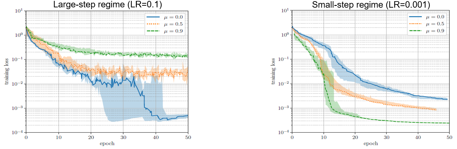

Fig.1 - Loss trajectory under the two regimes and different momentum values.

On the other hand, the two regimes inherit the same reaction to momentum from the generalization perspective.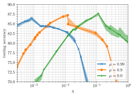

Fig.2 - Test accuracy under different learning rates $\eta$ and momentum values $\mu$.

Building upon the aforementioned two regimes, this paper proposes a new training scheme consisting of two stages: 1) using the large-step regime to target good generalization; 2) using the small-step regime coupled with large momentum to target good optimization. Also, they show an ablation study of the transition epoch between the first stage and the second stage, benchmarked against the aforementioned heuristic three-step learning rate schedule.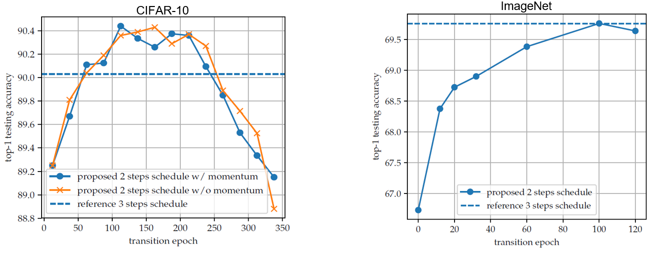

Fig.3 - Comparison between proposed schedule and the referenced classic three-step learning rate schedule.

Towards Explaining the Regularization Effect of Initial Large Learning Rate in Training Neural Networks: This paper shares the same motivation as the previous two-regime work, aiming to theoretically explain the effectiveness of an initial large learning rate and the annealing scheme. Its unique contribution is that it provides a concrete proof for the two-layer fully-connected network case.
Stiffness: A New Perspective on Generalization in Neural Networks: This paper investigates neural network training and generalization using the concept of stiffness. Specifically, it measures how stiff a network is by looking at how a small gradient step on one example affects the loss on another example. Given a data pair $(X, y)$, suppose the corresponding loss gradient can be represented as $\vec{g} = \nabla \mathbf{L} (f(X), y)$; we can then discuss the mutual influence between two independent data pairs, as shown in Fig. 4.

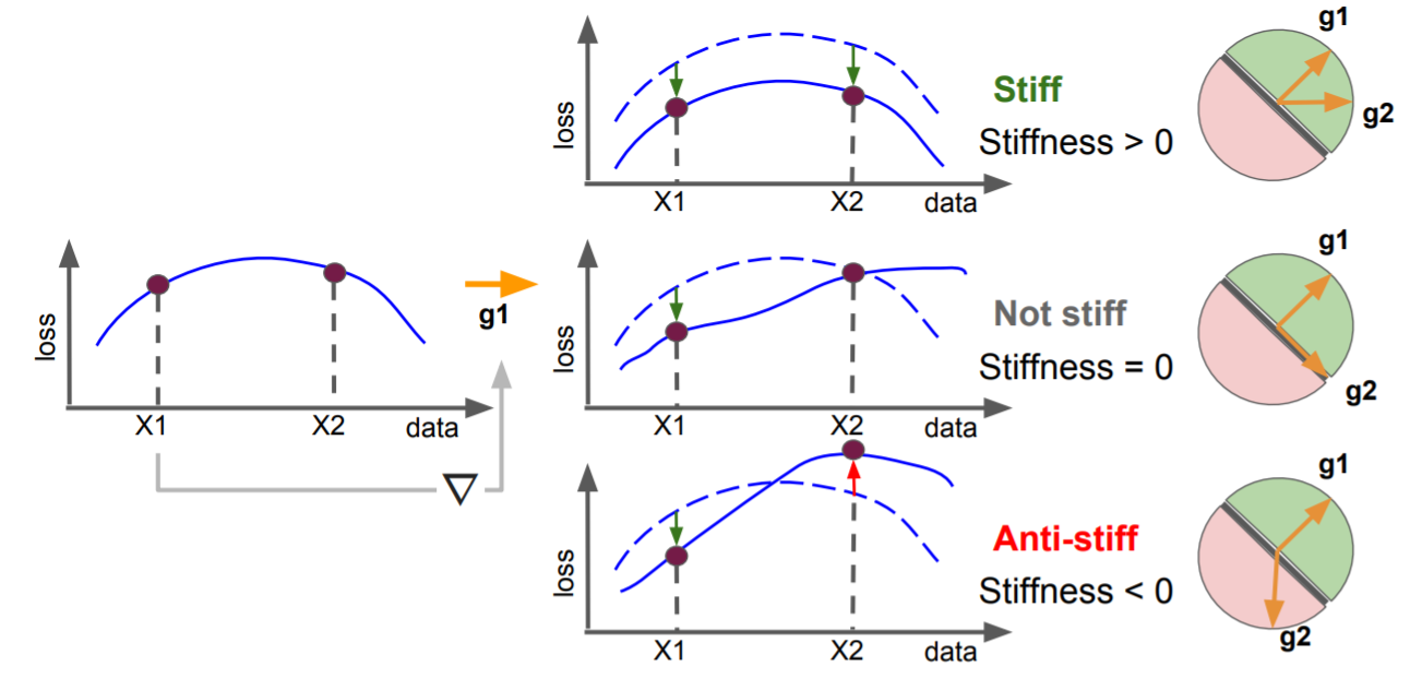
Fig.4 - A diagram illustrating the concept of stiffness. It can be viewed as the change in loss in an input induced by application of a gradient update based on another input. This is equivalent to the gradient alignment between gradients taken at the two inputs.

and then formulates the discrete (sign) or continuous (cos) stiffness metrics:

$S_{sign/cos}((X_1, y_1); (X_2, y_2); f) = \mathbb{E}[\text{sign/cos}(\vec{g_1} \cdot \vec{g_2})]$

Based on the proposed generalization metric, they visualize the change in stiffness between two data samples from the same or different classes, and find that the stiffness increases gradually during training, indicating an increasingly better generalization capability of the network. Moreover, they evaluate the stiffness between data samples from the training dataset and the validation dataset, and find that the proposed metric can identify whether the network is overfitting using only the training dataset. In particular, as illustrated in Fig. 5, when overfitting occurs, the stiffness measured both within the training dataset (train-train) and between the training and validation datasets (train-val) regresses to zero, which means we can tell when the network is overfitting without needing to validate, demonstrating that it is a good metric for quantifying generalization.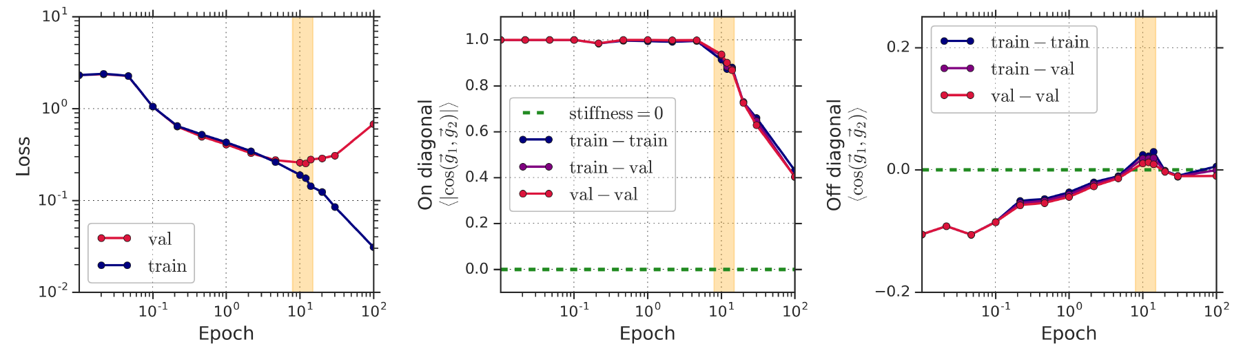

Fig.5 - The evolution of training and validation loss (left panel), within-class stiffness (central panel) and between-class stiffness (right panel) during training. The onset of over-fitting is marked in orange.

The Break-Even Point on Optimization Trajectories of Deep Neural Networks: This paper investigates how the hyperparameters of SGD used in the early phase of training affect the rest of the optimization trajectory. Before talking about the concrete analysis, we need to keep in mind two concepts:

1. ***Spectrum of the Hessian ($\lambda_H^1$)***: measures the local curvature of the loss surface

2. ***Spectrum of the Covariance of the Gradient ($\lambda_K^1$)***: measures the variance of the gradient

The first concept is the break-even point. Instead of understanding it through mathematical equations, here I provide an intuitive explanation: Assuming the spectral norm of the Hessian increases monotonically along the optimization trajectory, gradient descent reaches a point in the early phase of training at which it oscillates along the most curved direction of the loss surface; we call this point the break-even point. Specifically, the break-even point is where the spectral norm of the Hessian or the covariance of the gradient saturates. Before that point, the spectral norm increases monotonically; after that point, the spectral norm stays constant, meaning that the optimization enters a convex-like valley in the loss surface thereafter, and the trajectory oscillates along the most curved direction. Also, the break-even point occurs at a very early stage of network training.

Fig. 6 demonstrates that the assumption (the spectral norm increases monotonically) holds when training a simple CNN on CIFAR-10 under two different learning rate settings. It also indicates that the saturation values differ when using different hyperparameters.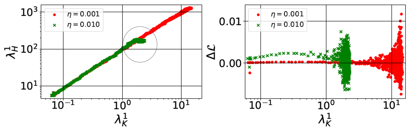

Fig.6 - The spectral norm of $H$ ($\lambda_H^1$, left) and $\Delta L$ (difference in the training loss computed between two consecutive steps, right) versus $\lambda_K^1$ at different training iterations.

Then, to probe how the hyperparameters of SGD used in the early phase of training matter, one can visualize the optimization trajectories under different hyperparameter settings in Fig. 7 (i.e., large/small learning rate here). At the beginning, the two settings are optimized from the same initialization and therefore share the same trajectory. After a while, their trajectories diverge in different directions until reaching the break-even points, while the large learning rate reaches a smaller $\lambda_K^1$ than its counterpart and shows good generalization thereafter.

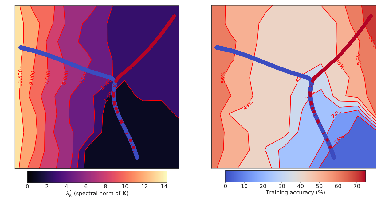
Fig.7 - Visualization of the early part of the training trajectories on CIFAR-10 before reaching 65% training accuracy (break-even point). Red line: LR=0.01; Blue line: LR=0.001.

Based on the break-even point observation, this paper proposes two conjectures to investigate the effects of different hyperparameters:

1. Along the SGD trajectory, the maximum attained values of $\lambda_H^1$ and $\lambda_K^1$ are smaller for a larger learning rate or a smaller batch size.

2. Along the SGD trajectory, the maximum attained values of $\lambda_H^\* / \lambda_H^1$ and $\lambda_K^\* / \lambda_K^1$ are larger for a larger learning rate or a smaller batch size.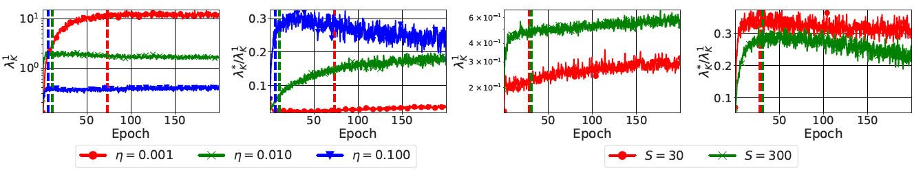

Fig.8 - The optimization trajectories corresponding to higher learning rates ($\eta$) or lower batch sizes ($S$).

On the Frequency Domain Perspective

Understanding the training process of Deep Neural Networks (DNN) is a fundamental problem in the area of deep learning. Here are the papers analyzing DNN training from the frequency domain perspective. The concept of “frequency” is central to understanding the papers below. In this context, “frequency” refers to response frequency, not image (or input) frequency, as explained below.

Training Behavior of Deep Neural Network in Frequency Domain: This paper analyzes the network training from the frequency perspective, aiming to claim the F-Principle: DNNs often fit target functions from low to high frequencies during the training process.

One of the difficulties of frequency analysis for image classification is how to compute the high-dimensional Fourier transform given a dataset $(x_k, y_k)$. They use the first principal component of the inputs $x_k = x_k \cdot v\_{PC}$. Then, using the Fourier transform, we can represent the dataset in the frequency domain:

$\mathbf{F}\_{PC}\[y\](\gamma) = \frac{1}{n} \sum\_{j=1}^{n-1} y\_j \cdot exp(-2\pi i x\_j \gamma)$

Where $\gamma$ is the frequency index. Suppose the network's prediction is $T(x_k)$; we then define the relative difference as:

$\Delta\_F(\gamma) = \frac{\|\mathbf{F}\_{PC}\[y\](\gamma) - \mathbf{F}\_{PC}\[T\](\gamma)\|}{\|\mathbf{F}\_{PC}\[y\](\gamma)\|}$

We can view the defined relative difference as the frequency loss, measuring the similarity between the frequencies of the ground truth and the predictions. This paper visualizes the changes in frequency loss at several selected frequency indices during training, as shown in Fig. 9.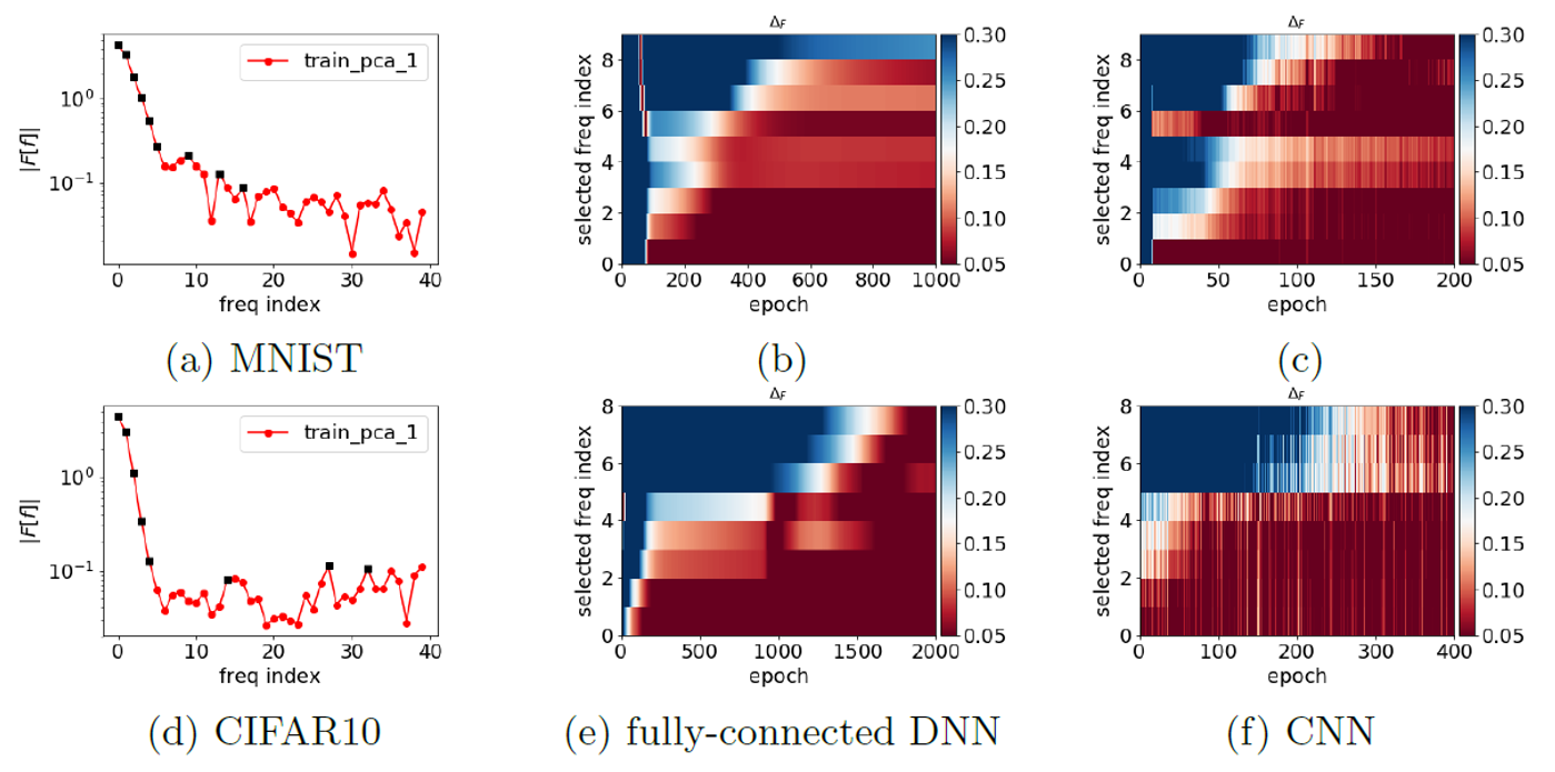

Fig.9 - Frequency analysis of the DNN output function along the first principal component during training. The training datasets for the first and second rows are from MNIST and CIFAR-10, respectively. The neural networks for the second and third columns are a fully-connected DNN and a CNN, respectively.

By examining the relative error of certain selected key frequency components (marked by black squares), one can clearly observe that DNNs of both structures, for both datasets, tend to capture the training data in order from low to high frequencies, as stated by the F-Principle.

On the Spectral Bias of Neural Networks: This paper shares the same motivation and claim as the F-Principle.

What happens during the early phase of DNN training

Similar to humans and animals, deep artificial neural networks exhibit critical periods, which correspond exactly to the early phase of training. A lot of phenomena have been discovered during the early phase of network training. For example, sparse, trainable sub-networks emerge, gradient descent moves into a small subspace, and the network undergoes a critical period. Two recent works are briefly introduced below.

Critical Learning Periods in Deep Networks: Researchers have documented critical periods affecting a range of species and systems; as machine learning researchers, it is natural to ask whether neural network training also experiences such critical periods. If so, when is the critical period? This paper answers that question using a deficit ablation study.

To explore whether critical periods exist in network training, this paper measures the test accuracy affected by the deficit as a function of the epoch $N$ at which the deficit is corrected. From Fig. 10, we can readily observe the existence of a critical period: if the blur is not removed within the first 40-60 epochs, the final performance is severely degraded compared to the baseline.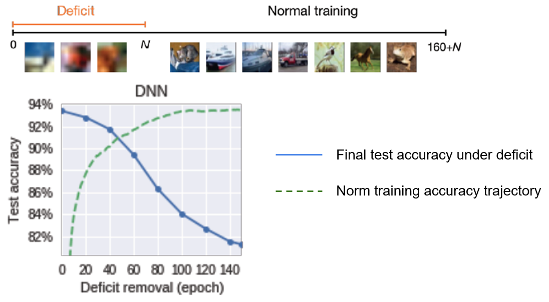

Fig.10 - Final test accuracy of a CNN trained with a cataract-like deficit as a function of the transition epoch at which the deficit is removed.

Further, to explore whether the critical period occurs in the early training phase, they conduct another ablation study on the deficit's starting epoch. The decrease in final performance can be used to measure the sensitivity to the deficit; the most sensitive epochs correspond to the early, rapid training phase. Afterwards, the network is largely unaffected by the temporary deficit.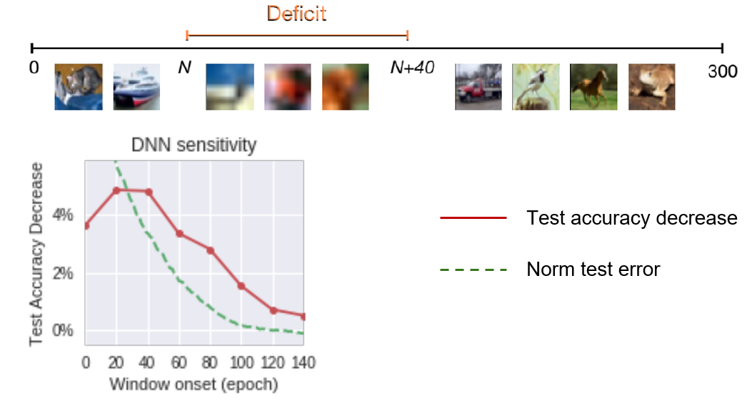

Fig.11 - The decrease in final performance of a CNN as a function of the onset of a short, 40-epoch deficit.

The Early Phase of Neural Network Training: Since the early stage of training is critical, this paper investigates it further, aiming to provide a unified framework for understanding the changes that DNNs undergo during this early phase of training.

They first provide a detailed statistical summary of the changes in the early training phase, taking ResNet-20 on CIFAR-10 as an example.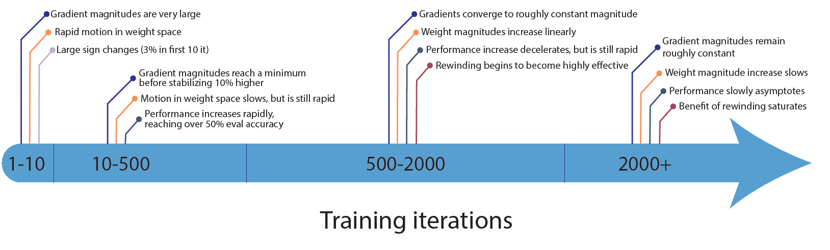

Fig.12 - Rough timeline of the early phase of training for ResNet-20 on CIFAR-10.

Among them, the most attractive phenomenon is that during 500-2000 iterations (2-10 epochs; 1/80-1/16 of the training stages), rewinding starts to be highly effective. Building upon the [Lottery Ticket Hypothesis (LTH)](https://arxiv.org/abs/1803.03635), something important happens during the early phase of training, such that when rewinding the network, one should rewind to these early phases instead of the initial phase. As demonstrated by Fig. 13, rewinding variants perform better than lottery initialization.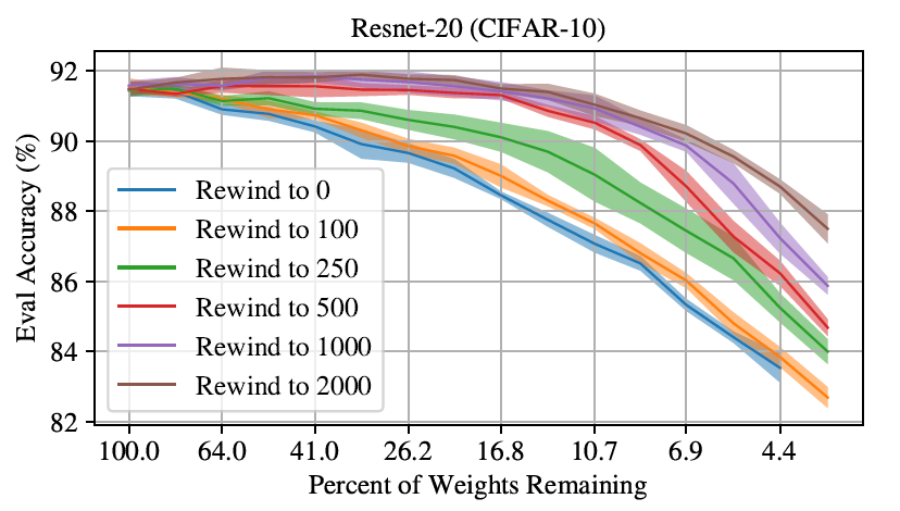

Fig.13 - Accuracy of IMP (Iterative Magnitude Pruning) when rewinding to various iterations of the early phase for ResNet-20 sub-networks as a function of sparsity level.

Then, they probe what is more important for the early phase of training: the signs of the weights or the magnitudes of the weights? By conducting ablation studies on weight signs and weight magnitudes from initialization or the early phase, this paper finds that both signs and magnitudes are important for handling highly sparse scenarios. Also, they probe whether the weights in the early phase can be sampled from a distribution by shuffling the weights globally or locally and then testing their performance in highly sparse scenarios. They find that the weights do not exhibit any clear distributional structure; thus, so far, the early phase of training remains the only way to obtain a good initialization for the retraining phase.